SQL Server Analysis Services (SSAS) Tutorial

Overview

SQL Server Analysis Services (SSAS) is the technology from the Microsoft Business Intelligence stack, to develop Online Analytical Processing (OLAP) solutions. In simple terms, you can use SSAS to create cubes using data from data marts / data warehouse for deeper and faster data analysis. 

Cubes are multi-dimensional data sources which have dimensions and facts (also known as measures) as its basic constituents. From a relational perspective dimensions can be thought of as master tables and facts can be thought of as measureable details. These details are generally stored in a pre-aggregated proprietary format and users can analyze huge amounts of data and slice this data by dimensions very easily. Multi-dimensional expression (MDX) is the query language used to query a cube, similar to the way T-SQL is used to query a table in SQL Server.

Simple examples of dimensions can be product / geography / time / customer, and similar simple examples of facts can be orders / sales. A typical analysis could be to analyze sales in Asia-pacific geography during the past 5 years. You can think of this data as a pivot table where geography is the column-axis and years is the row axis, and sales can be seen as the values. Geography can also have its own hierarchy like Country->City->State.  Time can also have its own hierarchy like Year->Semester->Quarter. Sales could then be analyzed using any of these hierarchies for effective data analysis.

A typical higher level cube development process using SSAS involves the following steps:

1) Reading data from a dimensional model
2) Configuring a schema in BIDS (Business Intelligence Development Studio)
3) Creating dimensions, measures and cubes from this schema
4) Fine tuning the cube as per the requirements
5) Deploying the cube

In this tutorial we will step through a number of topics that you need to understand in order to successfully create a basic cube. Our high level outline is as follows:

• Design and develop a star-schema
• Create dimensions, hierarchies, and cubes
• Process and deploy a cube
• Develop calculated measures and named sets using MDX
• Browse the cube data using Excel as the client tool

When you start learning SSAS, you should have a reasonable relational database background. But when you start working in a multi-dimensional environment, you need to stop thinking from a two-dimensional (relational database) perspective, which will develop over time.

In this tutorial, we will also try to develop an understanding of OLAP development from the eyes of an OLTP practitioner.

SSAS 2008 Tutorial: Understanding Analysis Services

The basic idea of OLAP is fairly simple. Let's think about that book ordering data for a moment. Suppose you want to know how many people ordered a particular book during each month of the year. You could write a fairly simple query to get the information you want. The catch is that it might take a long time for SQL Server to churn through that many rows of data.

And what if the data was not all in a single SQL Server table, but scattered around in various databases throughout your organization? The customer info, for example, might be in an Oracle database, and supplier information in a legacy xBase database. SQL Server can handle distributed heterogeneous queries, but they're slower.

What if, after seeing the monthly numbers, you wanted to drill down to weekly or daily numbers? That would be even more time-consuming and require writing even more queries.

This is where OLAP comes in. The basic idea is to trade off increased storage space now for speed of querying later. OLAP does this by precalculating and storing aggregates. When you identify the data that you want to store in an OLAP database, Analysis Services analyzes it in advance and figures out those daily, weekly, and monthly numbers and stores them away (and stores many other aggregations at the same time). This takes up plenty of disk space, but it means that when you want to explore the data you can do so quickly.

Later in the chapter, you'll see how you can use Analysis Services to extract summary information from your data. First, though, you need to familiarize yourself with a new vocabulary. The basic concepts of OLAP include:

• Cube
• Dimension table
• Dimension
• Hierarchy
• Level
• Fact table
• Measure
• Schema

Cube

The basic unit of storage and analysis in Analysis Services is the cube. A cube is a collection of data that's been aggregated to allow queries to return data quickly. For example, a cube of order data might be aggregated by time period and by title, making the cube fast when you ask questions concerning orders by week or orders by title.

Cubes are ordered into dimensions and measures. The data for a cube comes from a set of staging tables, sometimes called a star-schema database. Dimensions in the cube come from dimension tables in the staging database, while measures come from fact tables in the staging database.

Dimension table

A dimension table lives in the staging database and contains data that you'd like to use to group the values you are summarizing. Dimension tables contain a primary key and any other attributes that describe the entities stored in the table. Examples would be a Customers table that contains city, state and postal code information to be able to analyze sales geographically, or a Products table that contains categories and product lines to break down sales figures.

Dimension

Each cube has one or more dimensions, each based on one or more dimension tables. A dimension represents a category for analyzing business data: time or category in the examples above. Typically, a dimension has a natural hierarchy so that lower results can be "rolled up" into higher results. For example, in a geographical level you might have city totals aggregated into state totals, or state totals into country totals.

Hierarchy

A hierarchy can be best visualized as a node tree. A company's organizational chart is an example of a hierarchy. Each dimension can contain multiple hierarchies; some of them are natural hierarchies (the parent-child relationship between attribute values occur naturally in the data), others are navigational hierarchies (the parent-child relationship is established by developers.)

Level

Each layer in a hierarchy is called a level. For example, you can speak of a week level or a month level in a fiscal time hierarchy, and a city level or a country level in a geography hierarchy.

Fact table

A fact table lives in the staging database and contains the basic information that you wish to summarize. This might be order detail information, payroll records, drug effectiveness information, or anything else that's amenable to summing and averaging. Any table that you've used with a Sum or Avg function in a totals query is a good bet to be a fact table. The fact tables contain fields for the individual facts as well as foreign key fields relating the facts to the dimension tables.

Measure

Every cube will contain one or more measures, each based on a column in a fact table that you';d like to analyze. In the cube of book order information, for example, the measures would be things such as unit sales and profit.

Schema

Fact tables and dimension tables are related, which is hardly surprising, given that you use the dimension tables to group information from the fact table. The relations within a cube form a schema. There are two basic OLAP schemas: star and snowflake. In a star schema, every dimension table is related directly to the fact table. In a snowflake schema, some dimension tables are related indirectly to the fact table. For example, if your cube includes OrderDetails as a fact table, with Customers and Orders as dimension tables, and Customers is related to Orders, which in turn is related to OrderDetails, then you're dealing with a snowflake schema.

There are additional schema types besides the star and snowflake schemas supported by SQL Server 2008, including parent-child schemas and data-mining schemas. However, the star and snowflake schemas are the most common types in normal cubes.

SSAS 2008 Tutorial: Introducing Business Intelligence Development Studio

Business Intelligence Development Studio (BIDS) is a new tool in SQL Server 2008 that you can use for analyzing SQL Server data in various ways. You can build three different types of solutions with BIDS:

• Analysis Services projects
• Integration Services projects (you'll learn about SQL Server Integration Services in the SSIS 2008 tutorial)
• Reporting Services projects (you'll learn about SQL Server Reporting Services in the SSRS 2008 tutorial)

To launch Business Intelligence Development Studio, select Microsoft SQL Server 2008 > SQL Server Business Intelligence Development Studio from the Programs menu. BIDS shares the Visual Studio shell, so if you have Visual Studio installed on your computer, this menu item will launch Visual Studio complete with all of the Visual Studio project types (such as Visual Basic and C# projects).

SSAS 2008 Tutorial: Creating a Data Cube

To build a new data cube using BIDS, you need to perform these steps:

• Create a new Analysis Services project
• Define a data source
• Define a data source view
• Invoke the Cube Wizard

We'll look at each of these steps in turn.

You'll need to have the AdventureWorksDW2008 sample database installed to complete the examples in this chapter. This database is one of the samples that's available with SQL Server.

Creating a New Analysis Services Project

To create a new Analysis Services project, you use the New Project dialog box in BIDS. This is very similar to creating any other type of new project in Visual Studio.

Try It!

To create a new Analysis Services project, follow these steps:

1. Select Microsoft SQL Server 2008 > SQL Server Business Intelligence Development Studio from the Programs menu to launch Business Intelligence Development Studio.
2. Select File > New > Project.
3. In the New Project dialog box, select the Business Intelligence Projects project type.
4. Select the Analysis Services Project template.
5. Name the new project AdventureWorksCube1 and select a convenient location to save it.
6. Click OK to create the new project.

Figure 15-1 shows the Solution Explorer window of the new project, ready to be populated with objects.

Figure 15-1: New Analysis Services project

Defining a Data Source

A data source provides the cube's connection to the staging tables, which the cube uses as source data. To define a data source, you'll use the Data Source Wizard. You can launch this wizard by right-clicking on the Data Sources folder in your new Analysis Services project. The wizard will walk you through the process of defining a data source for your cube, including choosing a connection and specifying security credentials to be used to connect to the data source.

Try It!

To define a data source for the new cube, follow these steps:

1. Right-click on the Data Sources folder in Solution Explorer and select New Data Source.
2. Read the first page of the Data Source Wizard and click Next.
3. You can base a data source on a new or an existing connection. Because you don't have any existing connections, click New.
4. In the Connection Manager dialog box, select the server containing your analysis services sample database from the Server Name combo box.
5. Fill in your authentication information.
6. Select the Native OLE DB\SQL Native Client provider (this is the default provider).
7. Select the AdventureWorksDW2008 database. Figure 15-2 shows the filled-in Connection Manager dialog box.



Figure 15-2: Setting up a connection 

8. Click OK to dismiss the Connection Manager dialog box.
9. Click Next.
10. Select Use the Service Account impersonation information and click Next.
11. Accept the default data source name and click Finish.

Defining a Data Source View

A data source view is a persistent set of tables from a data source that supply the data for a particular cube. It lets you combine tables from as many data sources as necessary to pull together the data your cube needs. BIDS also includes a wizard for creating data source views, which you can invoke by right-clicking on the Data Source Views folder in Solution Explorer.

Try It!

To create a new data source view, follow these steps:

1. Right-click on the Data Source Views folder in Solution Explorer and select New Data Source View.
2. Read the first page of the Data Source View Wizard and click Next.
3. Select the Adventure Works DW data source and click Next. Note that you could also launch the Data Source Wizard from here by clicking New Data Source.
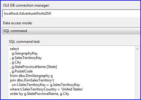
4. Select the FactFinance(dbo) table in the Available Objects list and click the > button to move it to the Included Object list. This will be the fact table in the new cube.
5. Click the Add Related Tables button to automatically add all of the tables that are directly related to the dbo.FactFinance table. These will be the dimension tables for the new cube. Figure 15-3 shows the wizard with all of the tables selected.


Figure 15-3: Selecting tables for the data source view

6. Click Next.
7. Name the new view Finance and click Finish. BIDS will automatically display the schema of the new data source view, as shown in Figure 15-4.

Figure 15-4: The Finance data source view

Invoking the Cube Wizard

As you can probably guess at this point, you invoke the Cube Wizard by right-clicking on the Cubes folder in Solution Explorer. The Cube Wizard interactively explores the structure of your data source view to identify the dimensions, levels, and measures in your cube.

Try It!

To create the new cube, follow these steps:

1. Right-click on the Cubes folder in Solution Explorer and select New Cube.
2. Read the first page of the Cube Wizard and click Next.
3. Select the option to Use Existing Tables.
4. Click Next.
5. The Finance data source view should be selected in the drop-down list at the top. Place a checkmark next to the FactFinance table to designate it as a measure group table and click Next.
6. Remove the check mark for the field FinanceKey, indicating that it is not a measure we wish to summarize, and click Next.
7. Leave all Dim tables selected as dimension tables, and click Next.
8. Name the new cube FinanceCube and click Finish.

Defining Dimensions

The cube wizard defines dimensions based upon your choices, but it doesn't populate the dimensions with attributes. You will need to edit each dimension, adding any attributes that your users will wish to use when querying your cube.

Try It!

1. In BIDS, double click on DimDate in the Solution Explorer.
2. Using Table 15-1 below as a guide, drag the listed columns from the right-hand panel (named Data Source View) and drop them in the left-hand panel (named Attributes) to include them in the dimension.
   
   

   DimDate

   CalendarYear

   CalendarQuarter

   MonthNumberOfYear

   DayNumberOfWeek

   DayNumberOfMonth

   DayNumberOfYear

   WeekNumberOfYear

   FiscalQuarter

   FiscalYear

   
   
   Table 15-1
   
3. Using Table 15-2, add the listed columns to the remaining four dimensions.
   

DimDepartmentGroup

DepartmentGroupName

DimAccount

AccountDescription

AccountType

DimScenario

ScenarioName

DimOrganization

OrganizationName

Table 15-2

Adding Dimensional Intelligence

One of the most common ways data gets summarized in a cube is by time. We want to query sales per month for the last fiscal year. We want to see production values year-to-date compared to last year's production values year-to-date. Cubes know a lot about time.

In order for SQL Server Analysis Services to be best able to answer these questions for you, it needs to know which of your dimensions stores the time information, and which fields in your time dimension correspond to what units of time. The Business Intelligence Wizard helps you specify this information in your cube.

Try It!                           

1. With your FinanceCube open in BIDS, click on the Business Intelligence Wizard button on the toolbar.
2. Read the initial page of the wizard and click Next.
3. Choose to Define Dimension Intelligence and click Next.
4. Choose DimDate as the dimension you wish to modify and click Next.
5. Choose Time as the dimension type. In the bottom half of this screen are listed the units of time for which cubes have knowledge. Using the Table 15-1 below, place a checkmark next to the listed units of time and then select which field in DimDate contains that type of data.
   

Time Property Name	Time Column
Year	CalendarYear
Quarter	CalendarQuarter
Month	MonthNumberOfYear
Day of Week	DayNumberOfWeek
Day of Month	DayNumberOfMonth
Day of Year	DayNumberOfYear
Week of Year	WeekNumberOfYear
Fiscal Quarter	FiscalQuarter
Fiscal Year	FiscalYear

Table 15-1:Time columns for FinanceCube
6. Click Next.

Hierarchies

You will also need to create hierarchies in your dimensions. Hierarchies are defined by a sequence of fields, and are often used to determine the rows or columns of a pivot table when querying a cube.

Try It!

1. In BIDS, double-click on DimDate in the solution explorer.
2. Create a new hierarchy by dragging the CalendarYear field from the left-hand pane (called Attributes) and drop it in the middle pane (called Hierarchies.)
3. Add a new level by dragging the CalendarQuarter field from the left-hand panel and drop it on the <new level> spot in the new hierarchy in the middle-panel.
4. Add a third level by dragging the MonthNumberOfYear field to the <new level> spot in the hierarchy.
5. Right-click on the hierarchy and rename it to Calendar.
6. Adding Dimensional IntelligenceIn the same manner, create a hierarchy named Fiscal that contains the fields FiscalYear, FiscalQuarter and MonthNumberOfYear. Figure 15-5 shows the hierarchy panel.

Figure 15-5: DimDate hierarchies

Deploying and Processing a Cube

At this point, you've defined the structure of the new cube - but there's still more work to be done. You still need to deploy this structure to an Analysis Services server and then process the cube to create the aggregates that make querying fast and easy.

To deploy the cube you just created, select Build > Deploy AdventureWorksCube1. This will deploy the cube to your local Analysis Server, and also process the cube, building the aggregates for you. BIDS will open the Deployment Progress window, as shown in Figure 15-5, to keep you informed during deployment and processing.

Try It!

To deploy and process your cube, follow these steps:

1. In BIDS, select Project > AdventureWorksCube1 from the menu system.
2. Choose the Deployment category of properties in the upper left-hand corner of the project properties dialog box.
3. Verify that the Server property lists your server name. If not, enter your server name. Click OK. Figure 15-6 shows the project properties window.

Figure 15-6: Project Properties
4. From the menu, select Build > Deploy AdventureWorksCube1. Figure 15-7 shows the Cube Deployment window after a successful deployment.

Figure 15-7: Deploying a cube

One of the tradeoffs of cubes is that SQL Server does not attempt to keep your OLAP cube data synchronized with the OLTP data that serves as its source. As you add, remove, and update rows in the underlying OLTP database, the cube will get out of date. To update the cube, you can select Cube > Process in BIDS.  You can also automate cube updates using SQL Server Integration Services, which you'll learn about in SSIS 2008 tutorial.

SSAS 2008 Tutorial: Exploring a Data Cube

At last you're ready to see what all the work was for. BIDS includes a built-in Cube Browser that lets you interactively explore the data in any cube that has been deployed and processed. To open the Cube Browser, right-click on the cube in Solution Explorer and select Browse. Figure 15-8 shows the default state of the Cube Browser after it's just been opened.

Figure 15-8: The cube browser in BIDS

The Cube Browser is a drag-and-drop environment. If you've worked with pivot tables in Microsoft Excel, you should have no trouble using the Cube browser. The pane to the left includes all of the measures and dimensions in your cube, and the pane to the right gives you drop targets for these measures and dimensions. Among other operations, you can:

• Drop a measure in the Totals/Detail area to see the aggregated data for that measure.
• Drop a dimension hierarchy or attribute in the Row Fields area to summarize by that value on rows.
• Drop a dimension hierarchy or attribute in the Column Fields area to summarize by that value on columns.
• Drop a dimension hierarchy or attribute in the Filter Fields area to enable filtering by members of that hierarchy or attribute.
• Use the controls at the top of the report area to select additional filtering expressions.

In fact, if you've worked with pivot tables in Excel, you'll find that the Cube Browser works exactly the same, because it uses the Microsoft Office PivotTable control as its basis.

Try It!

To see the data in the cube you just created, follow these steps:

1. Right-click on the cube in Solution Explorer and select Browse.
2. Expand the Measures node in the metadata panel (the area at the left of the user interface).
3. Expand the Fact Finance measure group.
4. Drag the Amount measure and drop it on the Totals/Detail area.
5. Expand the Dim Account node in the metadata panel.
6. Drag the Account Description attribute and drop it on the Row Fields area.
7. Expand the Dim Date node in the metadata panel.
8. Drag the Calendar hierarchy and drop it on the Column Fields area.
9. Click the + sign next to year 2001 and then the + sign next to quarter 3.
10. Expand the Dim Scenario node in the metadata panel.
11. Drag the Scenario Name attribute and drop it on the Filter Fields area.
12. Click the dropdown arrow next to scenario name. Uncheck all of the checkboxes except for the one next to the Budget value.

Figure 15-9 shows the result. The Cube Browser displays month-by-month budgets by account for the third quarter of 2001. Although you could have written queries to extract this information from the original source data, it's much easier to let Analysis Services do the heavy lifting for you.

Figure 15-9: Exploring cube data in the cube browser

SSAS 2008 Tutorial: Exercises

Although cubes are not typically created with such a single purpose in mind, your task is to create a data cube, based on the data in the AdventureWorksDW2008 sample database, to answer the following question: what were the internet sales by country and product name for married customers only?

Solutions to Exercises

To create the cube, follow these steps:

1. Select Microsoft SQL Server 2008 „ SQL Server Business Intelligence Development Studio from the Programs menu to launch Business Intelligence Development Studio.
2. Select File > New > Project.
3. In the New Project dialog box, select the Business Intelligence Projects project type.
4. Select the Analysis Services Project template.
5. Name the new project AdventureWorksCube2 and select a convenient location to save it.
6. Click OK to create the new project.
7. Right-click on the Data Sources folder in Solution Explorer and select New Data Source.
8. Read the first page of the Data Source Wizard and click Next.
9. Select the existing connection to the AdventureWorksDW2008 database and click Next.
10. Select Service Account and click Next.
11. Accept the default data source name and click Finish.
12. Right-click on the Data Source Views folder in Solution Explorer and select New Data Source View.
13. Read the first page of the Data Source View Wizard and click Next.
14. Select the Adventure Works DW2008 data source and click Next.
15. Select the FactInternetSales(dbo) table in the Available Objects list and click the > button to move it to the Included Object list.
16. Click the Add Related Tables button to automatically add all of the tables that are directly related to the dbo.FactInternetSales table. Also add the DimGeography dimension.
17. Click Next.
18. Name the new view InternetSales and click Finish.
19. Right-click on the Cubes folder in Solution Explorer and select New Cube.
20. Read the first page of the Cube Wizard and click Next.
21. Select the option to Use Existing Tables.
22. Select FactInternetSales and FactInternetSalesReason tables as the Measure Group Tables and click Next.
23. Leave all measures selected and click Next.
24. Leave all dimensions selected and click Next.
25. Name the new cube InternetSalesCube and click Finish.
26. In the Solution Explorer, double click the DimCustomer dimension.
27. Add the MaritalStaus field as an attribute, along with any other fields desired.
28. Similarly, edit the DimSalesTerritory dimension, adding the SalesTerritoryCountry field along with any other desired fields.
29. Also edit the DimProduct dimension, adding the EnglishProductName field along with any other desired fields.
30. Select Project > AdventureWorksCube2 Properties and verify that your server name is correctly listed. Click OK.
31. Select Build > Deploy AdventureWorksCube2.
32. Right-click on the cube in Solution Explorer and select Browse.
33. Expand the Measures node in the metadata panel.
34. Drag the Order Quantity and Sales Amount measures and drop it on the Totals/Detail area.
35. Expand the Dim Sales Territory node in the metadata panel.
36. Drag the Sales Territory Country property and drop it on the Row Fields area.
37. Expand the Dim Product node in the metadata panel.
38. Drag the English Product Name property and drop it on the Column Fields area.
39. Expand the Dim Customer node in the metadata panel.
40. Drag the Marital Status property and drop it on the Filter Fields area.
41. Click the dropdown arrow next to Marital Status. Uncheck the S checkbox.

Figure 15-10 shows the finished cube.

Building Your First Data Cube

Building Your First Cube

You can get a feel for what it takes to use SQL Server Analysis Services by building a cube based on the AdventureWorks data warehouse. Once you’ve had a chance to poke around there, you can take a look at some of the other ways of providing BI reporting.

NOTE: For this example, you’ll be working within the SQL Server Data Tools, or SSDT. Note that SSDT is entirely different from the SQL Server Management Studio that you’ve been mostly working with thus far. The SQL Server Data Tools is a different work area that is highly developer- (rather than administrator-) focused; indeed, it is a form of Visual Studio that just has project templates oriented around many of the “extra” services that SQL Server offers. In addition to the work you’ll do with SSDT in this chapter, you will also visit it some to work with Reporting Services, Integration Services, and more Analysis Services in the chapters ahead.

Try It Out: Creating an SSAS Project in SSDT

This is one of the most advanced examples in the book, so get ready for some fun. You’ll build a cube in SSAS, which gives you high-speed multidimensional analysis capability. This one will use UDM, but you’ll get a chance to use BISM in a little bit. Building your cube will require several steps: You’ll need to build a data source, a data source view, some dimensions, and some measures before your cube can be realized.

Start a New Project

To build an SSAS cube, you must first start a project by following these steps:

1. Open the SQL Server Data Tools and create a new project.
2. In the New Project dialog box under Installed Templates on the left, choose Business Intelligence Analysis Services.
3. In the main pane, select Analysis Services Multidimensional and Data Mining Project, as you can see in Figure 18-2.
   
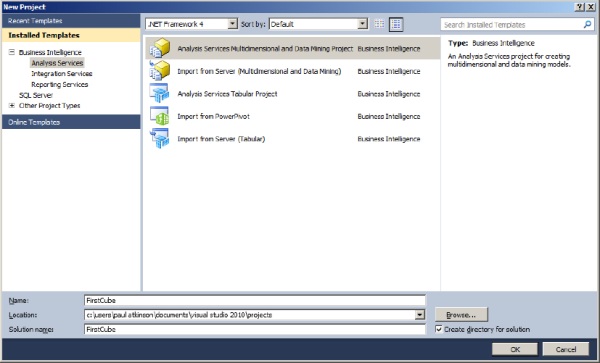   Figure 18-2. The New Project dialog with Analysis Services Multidimensional and Data Mining Project selected
4. 4. Name your project FirstCube and click OK.

You’re now presented with an empty window, which seems like a rare beginning to a project with a template; really, you have nothing to start with, so it’s time to start creating. The first component you’ll need is somewhere to retrieve data from: a data source.

Building a Data Source

To create the data source you’ll use for your first cube, follow these steps:

1. Navigate to the Solution Explorer pane on the right, right-click Data Sources, and click New Data Source. This will bring up the Data Source Wizard, which will walk you through the creation process just as you’d expect.
2. Before you skip by the opening screen as you usually would, though, take note of what it says (just this once. . .you can skip it later). I won’t re-type it here, but it’s giving you a heads-up about the next component you’ll create: the data source view.
3. Meanwhile, go ahead and click Next to continue creating your data source. In this next screen, it’s time to set up a connection string.
4. If your AdventureWorksDW database is visible as a selection already, go ahead and choose it; if not, click New.
5. For your server name, enter (local), and then drop down the box labeled Select or Enter a Database Name and choose AdventureWorksDW.
6. Click OK to return to the wizard and then click Next.
7. You can now enter the user you want SSAS to impersonate when it connects to this data source. Select Use the Service Account and click Next. Using the service account (the account that runs the SQL Server Analysis Server service) is fairly common even in production, but make sure that service account has privileges to read your data source.
8. For your data source name, type AdventureWorksDW and then click Finish.

Building a Data Source View

Now that you’ve created a data source, you’ll need a data source view (as the Data Source Wizard suggested). Follow these steps:

1. Right-click Data Source Views and choose New Data Source View. Predictably, up comes the Data Source View Wizard to walk you through the process. Click Next.
2. Make sure the AdventureWorksDW data source is selected and then click Next.
3. On the Select Tables and Views screen, choose FactInternetSales under Available objects and then click the right arrow to move it into the Included Objects column on the right.
4. To add its related dimensions, click the Add Related Tables button as shown in Figure 18-3 and then click Next. Note that one of the related tables is a fact, not a dimension. There’s no distinction made at this level. Later, you will be able to select and edit dimensions individually.
   
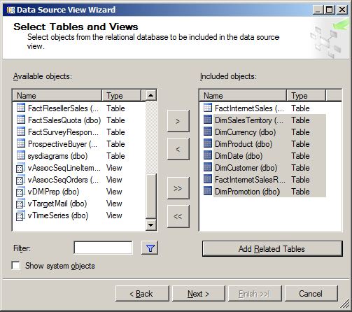   Figure 18-3. Adding tables to the view
5. On the last screen, name your data source view according to its contents: Internet Sales.
6. Click Finish to create the Internet Sales data source view, and you’ll see it in the content pane, looking something like Figure 18-4 (your exact layout may vary).
   
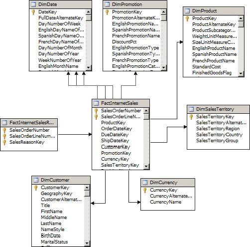   Figure 18-4. The finished Internet Sales view

Creating Your First Cube

Now for the exciting part…you get to create your first cube.

1. Right-click Cubes in the Solution Explorer and select New Cube to bring up the Cube Wizard. This will walk you through choosing measure groups (which you currently know as fact tables), the measures within them, and your dimensions for this cube. Don’t worry about the word “cube” here and think you just have to stick with three dimensions, either; cube is just a metaphor, and you can create a four-dimensional hypercube, a tesseract, or an unnamed higher-dimensional object if you want (and you’re about to do so!). To begin, click Next.
2. On the Select Creation Method screen, make sure Use Existing Tables is selected, and click Next.
3. The wizard will now want you to tell it where to find measure groups. You could help it out by telling it those are in your fact tables, but never mind — it’s smart enough to figure it out. If you click Suggest, it will automatically select the correct tables. Do so (the result is shown in Figure 18-5) and then click Next.
   
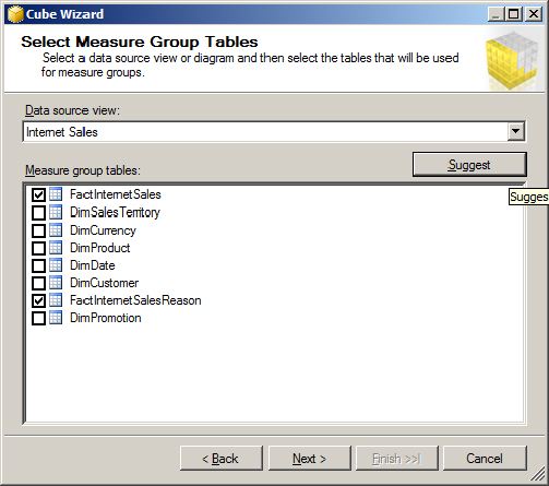   Figure 18-5. Selecting Measure Group Tables
4. Now the wizard would like to know which measures from your measure groups (fact tables) you’d like to store in the cube. By default it’s got them all selected; go ahead and accept this by clicking Next.
5. At this point, you have measures, but you still need dimensions; the wizard will select the dimension tables from your data source view and invite you to create them as new dimensions in the UDM. Again, by default they’re all selected, and you can click Next.
6. The wizard is now ready to complete. Verify you have something that looks like Figure 18-6, and go back to make corrections if you need. If everything appears to be in order, click Finish.
   
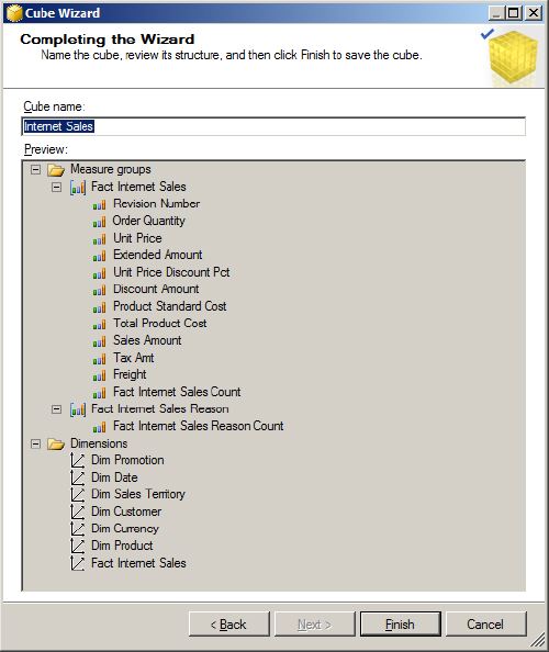   Figure 18-6. Completing the Cube Wizard

Making Your Cube User-Friendly

Right about now, you’re probably expecting something like “congratulations, you’re done!” After all, you’ve built up the connection, designated the measures and dimensions, and defined your cube, so it would be nifty if you could just start browsing it, but you’re not quite there yet. First you’ll want to make some of your dimensions a little more friendly; they’re currently just defined by their keys because SSAS doesn’t know which fields in your dimension tables to use as labels. Once you’ve settled that, you’ll need to deploy and process your cube for the first time before it’s ready to use.

1. In the Solution Explorer under Dimensions, double-click DimDate. The Dimension Editor will come up, allowing you to make this dimension a bit more useable.
2. To make the date attributes available, highlight all of them (except DateKey, which as you can see is already in the attribute list) and drag them to the attribute list.
3. Date, of course, is a dimension that can be naturally defined as a hierarchy (like you did quite manually in the T-SQL grouping examples). Drag Fiscal Quarter from the Attributes pane to the Hierarchies pane to start creating a hierarchy.
4. Drag Month Number of Year to the tag under Fiscal Quarter, and DateKey similarly below that.
5. Finally, rename the hierarchy (right-click it and choose Rename) to Fiscal Quarter - Month. The result should look something like Figure 18-7.
   
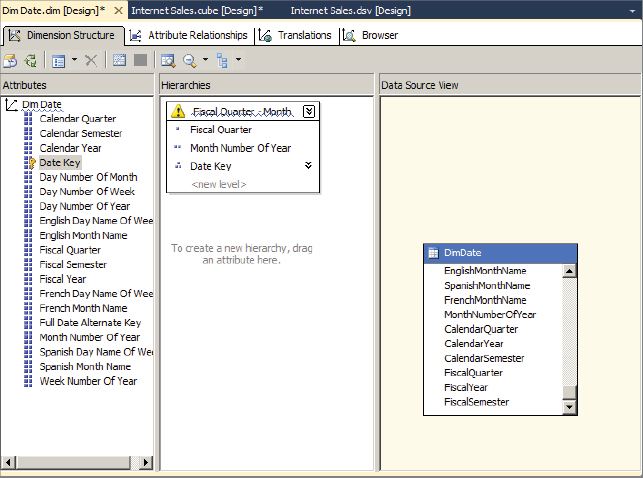   Figure 18-7. Renaming The Hierarchy
6. Save the DimDate dimension and close the dimension editor. You will be prompted to save changes to your cube along with the new dimension changes; do so.
7. For each of the other dimensions, don’t create hierarchies for now, but bring all the interesting text columns into the Attributes pane (you can bring over all the non-key columns except for the Large Photo column in the Products table), and re-save the dimensions.

Deploying the Cube

There’s more you can do to create useful hierarchies, but for now it’s time to build, deploy, and process the cube. This process can be started by following these steps.

1. Select Deploy First Cube on the Build menu. You’ll see a series of status messages as the cube is built, deployed, and processed for the first time. You’ll receive a few warnings when you deploy FirstCube, and if they’re warnings and not errors, you can safely ignore them for now.
2. When it’s done and you see Deployment Completed Successfully in the lower right, your first cube is ready to browse.

NOTE When you set up a user in your data source view, you chose the service user — this is the user that’s running the Analysis Services service. If that user doesn’t have a login to your SQL Server, you’re going to receive an error when you try to process your cube.

In addition, this example bypasses a step that’s important for processing hierarchies in cubes with large amounts of data: creating attribute relationships. The cube will still successfully process (though you will receive a warning), and for the data volumes in the AdventureWorksDW database it will perform adequately. For larger data volumes, you will need to address this warning. For more information on how to do that, consult the more complete SSAS text.

3. In the Solution Explorer pane, double-click the Internet Sales cube and then look in the tabs above the main editing pane for the Browser tab and click that.
4. Now you can drag and drop your measures (such as ExtendedAmount) and your dimensions and hierarchies (look for the Fiscal Quarter - Month hierarchy under the Due Date dimension) into the query pane, and voilà — your data is sliced and diced as quickly as you please.

How It Works

Whew! That was a lot of setup, but the payoff is pretty good too. What you’ve done is to build your first cube, and under the hood you’ve created a UDM-based semantic model queryable through the MDX language. This cube isn’t fully complete — you’d probably want to add some aggregations, attribute relationships, and other elements, but it’s an impressive start.

It started when you chose your project type. The Multidimensional project types build the UDM-based data models, whereas the Tabular Project types build your model in BISM. Because I plan to bring you through PowerPivot shortly (which is BISM-based), I led you down the UDM route here. You’ll find that for basic operations the two are equally capable.

Once you had your project put together, you had a few components to create on the way to browsing your cube. Let’s call a few out.

• Data source: Your data source is a connection to an individual place where data for your BI reporting can be found. While this one was a SQL Server data source, you can use any number of providers, both included and third-party. Nothing here should surprise you too much; this is a similar kind of list to what you’d find in SSIS, for example.
• Data source views: A data source view is a much more interesting animal. Using a data source, the data source view contains a set of tables or views, and defines the relationships among them. Each DSV is usually built around a business topic, and contains any tables related to that topic.
• Cubes: While the next thing you proceeded to create was a cube, the Cube Wizard went ahead and built measure groups and dimensions for you along the way. Without those, you haven’t got much of a cube. The cube isn’t a pass-through directly to your source data. To update the data in the cube, you must process the cube; you can do this through a regularly scheduled job with SQL Agent or, of course, manually. In this case, the wizard took care of a lot of the details for you, but you’ll read more about what the cube really is in a few minutes.

SQL Server Integration Services (SSIS) Tutorial

OverviewSQL Server Integration Services (SSIS) is a tool that we use to perform ETL operations; i.e. extract, transform and load data.  While ETL processing is common in data warehousing (DW) applications, SSIS is by no means limited to just DW; e.g. when you create a Maintenance Plan using SQL Server Management Studio (SSMS) an SSIS package is created.  At a high level, SSIS provides the ability to:

• retrieve data from just about any source
• perform various transformations on the data; e.g. convert from one type to another, convert to uppercase or lowercase, perform calculations, etc.
• load data into just about any source
• define a workflow

The first version of SSIS was released with SQL Server 2005.  SSIS is a replacement for Data Transformation Services (DTS) which was available with SQL Server 7.0 and SQL Server 2000.  SSIS builds on the capabilities introduced with DTS.

In this tutorial we will step through a number of topics that you need to understand in order to successfully build an SSIS package.  Our high level outline is as follows:

• Creating SSIS packages with SQL Server Management Studio (SSMS)
• Business Intelligence Development Studio (BIDS)
• Creating a simple SSIS package in BIDS
• Deploying SSIS packages
• Executing SSIS packages

Overview
In this section we will walk through creating a simple SSIS package from scratch.  As an example we will generate an Excel spreadsheet that can be used to manually enter a sales forecast by city and state.  The city and state information will be extracted from the AdventureWorksDW database and output to an Excel spreadsheet.  The sales department could use this spreadsheet to enter the forecast.  Another SSIS package will import the data from the spreadsheet and update a table in the AdventureWorksDW database.

In the sections that follow we will walk through the following steps:

• Create a new SSIS package and discuss some of the package properties
• Add Connection Managers for our data source and destination
• Add tasks to the package Control Flow
• Add tasks to the package Data Flow
• Execute the package in BIDS

---

SQL Server Integration Services (SSIS) Data Flow

OverviewThis is our fourth step in creating a simple SSIS package from scratch.  In this section we will take a look at the Data Flow designer which contains the various tasks that will be performed by a Data Flow task specified in the Control Flow. 

ExplanationTo begin launch BIDS by selecting SQL Server Business Intelligence Development Studio from the Microsoft SQL Server program group.  Click File, Open, Project / Solution on the top level menu to display the Open Project dialog.  Navigate to the location of the solution as shown below then click Open:

Expand the SSIS Packages node under the Tutorial-Sample-1 project in Solution Explorer and you will see the following:

Double click on the SSIS package CreateSalesForecastInput.dtsx to open the package.  Click on the Data Flow tab in the designer and you should see the empty Data Flow designer as shown below:

The Toolbox will now display the tasks that are available in the Data Flow as shown below:

As you can see there are quite a few built-in tasks available.  For our current package we want to retrieve some data from the AdventureWorksDW database and output it to an Excel spreadsheet.  To do this we need an OLE DB Source and an Excel Destination.  In addition we need to add a column to the Data Flow; this column will be the numeric column in the spreadsheet where the user enters the forecast amount.  Drag and drop an OLE DB Source, Derived Column, and Excel Destination from the Toolbox onto the Data Flow designer.  After doing so the Data Flow designer should look like this:

The red icons inside of the tasks are an indicator that there is some configuration required.  Right click on the OLE DB Source then select Edit from the popup menu.  This will open the OLE DB Source Editor on the Connection Manager page.  Fill in the dialog as shown below:

We setup the OLD DB connection manager in the Connection Managers step earlier.  The SQL command text contains a simple query to retrieve the list of cities and states in the United States.

Click on Columns to display the column mappings as shown below:

By default all columns returned from the query are selected and the Output Column names are the same.  The Output Column names can be edited; we will leave them as is.  Click OK to complete the OLE DB Source Editor.  You will now see a green and a red line dangling from the OLE DB Source task on the Data Flow designer.  The green line is the normal data flow; the red line is the error flow.  Drag the green line and connect it to the Derived Column task as shown below:

Notice that the red icon is now gone from the OLE DB Source task and it is now properly configured.

The Derived Column task allows us to add a column to the Data Flow.  Right click on it, select Edit, then fill in the Derived Column transformation Editor as shown below:

We have now added a new currency column to the data flow with a name of Forecast, and a value of 0.  Click on the Derived Column task and drag the green arrow to connect to the Excel Destination task.

Right click the Excel Destination task and select Edit from the popup menu.  The Excel Destination Editor dialog will be displayed.  Click the New button next to the Name of the Excel Sheet to display the Create Table dialog as shown below:

The Create Table dialog allows us to create a new table in the Excel spreadsheet.  The columns and their types are determined by the data flow.  We configured an OLE DB Source task that executes a query and a Derived Column task that added the Forecast column to the data flow.  You can edit the CREATE TABLE script if you like.  Click OK on the Create Table dialog and the Excel Destination Editor Connection Manager page will look like this:

We configured the Excel Connection Manager in step two of this tutorial.  Click on Mappings to display the Mappings page as shown below:

The above dialog sets the Destination Column names to the Input Column names by default.

At this point we have completed the Data Flow. Note that there are no longer any red icons in the task rectangles. We will proceed to the final step in this section of the tutorial and execute the package.

SSIS Tutorial: Creating a Simple ETL Package

Microsoft SQL Server Integration Services (SSIS) is a platform for building high performance data integration solutions, including extraction, transformation, and load (ETL) packages for data warehousing. SSIS includes graphical tools and wizards for building and debugging packages; tasks for performing workflow functions such as FTP operations, executing SQL statements, and sending e-mail messages; data sources and destinations for extracting and loading data; transformations for cleaning, aggregating, merging, and copying data; a management service, the Integration Services service for administering package execution and storage; and application programming interfaces (APIs) for programming the Integration Services object model.

In this tutorial, you will learn how to use SSIS Designer to create a simple Microsoft SQL Server Integration Services package. The package that you create takes data from a flat file, reformats the data, and then inserts the reformatted data into a fact table. In following lessons, the package is expanded to demonstrate looping, package configurations, logging and error flow.

When you install the sample data that the tutorial uses, you also install the completed versions of the packages that you will create in each lesson of the tutorial. By using the completed packages, you can skip ahead and begin the tutorial at a later lesson if you like. If this is your first time working with packages or the new development environment, we recommend that you begin with Lesson1.

Administer a Report Server Database (SSRS Native Mode)

Report Server Database (SSRS Native Mode)

A report server is a stateless server that uses the SQL Server Database Engine to store metadata and object definitions. A native mode Reporting Services installation uses two databases to separate persistent data storage from temporary storage requirements. The databases are created together and bound by name. By default, the database names are reportserver and reportservertempdb, respectively.

A SharePoint mode Reporting Services installation will also create a database for the data alerting feature. The three databases in SharePoint mode are associated with Reporting Services service applications. For more information, see Manage a Reporting Services SharePoint Service Application

The databases can run on a local or remote Database Engine instance. Choosing a local instance is useful if you have sufficient system resources or want to conserve software licenses, but running the databases on a remote computer can improve performance.

You can port or reuse an existing report server database from previous installation or a different instance with another report server instance. The schema of the report server database must be compatible with the report server instance. If the database is in an older format, you will be prompted to upgrade it to the current format. Newer versions cannot be down graded to an older version. If you have a newer report server database, you cannot use it with an earlier version of a report server instances. For more information about how report server databases are upgraded to newer formats, see Upgrade a Report Server Database.

Report Server Database

The report server database is a SQL Server database that stores the following content:

• Items managed by a report server (reports and linked reports, shared data sources, report models, folders, resources) and all of the properties and security settings that are associated with those items.
• Subscription and schedule definitions.
• Report snapshots (which include query results) and report history.
• System properties and system-level security settings.
• Report execution log data.
• Symmetric keys and encrypted connection and credentials for report data sources.

Because the report server database stores application state and persistent data, you should create a backup schedule for this database to prevent data loss. For recommendations and instructions on how to back up the database, see Moving the Report Server Databases to Another Computer (SSRS Native Mode).

Report Server Temporary Database

Each report server database uses a related temporary database to store session and execution data, cached reports, and work tables that are generated by the report server. Background server processes will periodically remove older and unused items from the tables in the temporary database.

Reporting Services does not re-create the temporary database if it is missing, nor does it repair missing or modified tables. Although the temporary database does not contain persistent data, you should back up a copy of the database anyway so that you can avoid having to re-create it as part of a failure recovery operation.

If you back up the temporary database and subsequently restore it, you should delete the contents. Generally, it is safe to delete the contents of the temporary database at any time. However, you must restart the Report Server Windows service after you delete the contents

Create a Report Server Database (SSRS Configuration Manager)

Reporting Services Native mode uses two SQL Server relational databases to store report server metadata and objects. One database is used for primary storage, and the second one stores temporary data. The databases are created together and bound by name. With a default SQL Server instance, the databases are named reportserver and reportservertempdb. Collectively, the two databases are referred to as the "report server database" or "report server catalog".

Reporting Services SharePoint mode includes a third database that is used for data alerting metadata. The three databases are created for each Reporting Services service application and the database names by default include a guid that represents the service application. The following are example names of the three SharePoint mode databases:

• ReportingService_90a9f37075544f22953c4a62e4a9f370
• ReportingService_90a9f37075544f22953c4a62e4a9f370TempDB
• ReportingService_90a9f37075544f22953c4a62e4a9f370_Alertin

Ways to Create the Report Server Database

Native Mode: You can create the Native mode report server database in the following ways:

• Automatically: Use SQL Server Setup Wizard, if you choose the default configuration installation option. In the SQL Server Installation Wizard, this is the Install and configure in the Report Server Installation Options page. If you chose the Install only option, you must use the Reporting Services Configuration Manager to create the database.
• Manually: Use the Reporting Services Configuration Manager. You must create the report server database manually if you are using a remote SQL Server Database Engine to host the database. For more information, see Create a Native Mode Report Server Database (SSRS Configuration Manager).

SharePoint Mode: The Report Server Installation Options page only has one option for SharePoint mode of Install Only. This option installs all the Reporting Services files and the Reporting Services shared service. The next step is to create at least one Reporting Services service application in one of the following ways:

• Use SharePoint Central Administration to create a Reporting Services service application. For more information see the “Service Application” section of Step 3: Create a Reporting Services Service Application.
• Use Reporting Services PowerShell cmdlets to create a service application and the report server databases. For more information see the sample for creating service applications in the topic PowerShell cmdlets for Reporting Services SharePoint Mode.
• 
  

Create a Report Server Database (SSRS Configuration Manager)

SQL Server 2016

Other Versions

 

Applies To: SQL Server 2016 Preview

Reporting Services Native mode uses two SQL Server relational databases to store report server metadata and objects. One database is used for primary storage, and the second one stores temporary data. The databases are created together and bound by name. With a default SQL Server instance, the databases are named reportserver and reportservertempdb. Collectively, the two databases are referred to as the "report server database" or "report server catalog".

Reporting Services SharePoint mode includes a third database that is used for data alerting metadata. The three databases are created for each Reporting Services service application and the database names by default include a guid that represents the service application. The following are example names of the three SharePoint mode databases:

• ReportingService_90a9f37075544f22953c4a62e4a9f370
• ReportingService_90a9f37075544f22953c4a62e4a9f370TempDB
• ReportingService_90a9f37075544f22953c4a62e4a9f370_Alerting

Important

Do not write applications that run queries against the report server database. The report server database is not a public schema. The table structure might change from one release to the next. If you write an application that requires access to the report server database, always use the Reporting Services APIs to access the report server database. The exception to this are the execution log views. For more information, see Report Server Execution Log and the ExecutionLog3 View

Ways to Create the Report Server Database

Native Mode: You can create the Native mode report server database in the following ways:

• Automatically: Use SQL Server Setup Wizard, if you choose the default configuration installation option. In the SQL Server Installation Wizard, this is the Install and configure in the Report Server Installation Options page. If you chose the Install only option, you must use the Reporting Services Configuration Manager to create the database.
• Manually: Use the Reporting Services Configuration Manager. You must create the report server database manually if you are using a remote SQL Server Database Engine to host the database. For more information, see Create a Native Mode Report Server Database (SSRS Configuration Manager).

SharePoint Mode: The Report Server Installation Options page only has one option for SharePoint mode of Install Only. This option installs all the Reporting Services files and the Reporting Services shared service. The next step is to create at least one Reporting Services service application in one of the following ways:

• Use SharePoint Central Administration to create a Reporting Services service application. For more information see the “Service Application” section of Step 3: Create a Reporting Services Service Application.
• Use Reporting Services PowerShell cmdlets to create a service application and the report server databases. For more information see the sample for creating service applications in the topic PowerShell cmdlets for Reporting Services SharePoint Mode.

Database Server Version Requirements

SQL Server is used to host the report server databases. The SQL Server Database Engine instance can be a local or remote instance. The following are the supported versions of SQL Server Database Engine that can be used to host the report server databases:

• SQL Server 2016 Community Technology Preview 2 (CTP2)
• SQL Server 2014
• SQL Server 2012
• SQL Server 2008 R2
• SQL Server 2008
• SQL Server 2005

Creating the report server database on a remote computer requires that you configure the connection to use a domain user account or a service account that has network access. If you decide to use a remote SQL Server instance, consider carefully which credentials the report server should use to connect to the SQL Server instance. For more information, see Configure a Report Server Database Connection (SSRS Configuration Manager).

Moving the Report Server Databases to Another Computer (SSRS Native Mode)

You can move the report server databases that are used in an installation SQL Server Database Engine to an instance that is on a different computer. Both the reportserver and reportservertempdb databases must be moved or copied together. A Reporting Services installation requires both databases; the reportservertempdb database must be related by name to the primary reportserver database you are moving.

Applies to: Reporting Services Native mode.

Moving a database does not effect scheduled operations that are currently defined for report server items.

• Schedules will be recreated the first time that you restart the Report Server service.
• SQL Server Agent jobs that are used to trigger a schedule will be recreated on the new database instance. You do not have to move the jobs to the new computer, but you might want to delete jobs on the computer that will no longer be used.
• Subscriptions, cached reports, and snapshots are preserved in the moved database. If a snapshot is not picking up refreshed data after the database is moved, clear the snapshot options in Report Manager, click Apply to save your changes, re-create the schedule, and click Applyagain to save your changes.
• Temporary report and user session data that is stored in reportservertempdb are persisted when you move that database.

SQL Server provides several approaches for moving databases, including backup and restore, attach and detach, and copy. Not all approaches are appropriate for relocating an existing database to a new server instance. The approach that you should use to move the report server database will vary depending on your system availability requirements. The easiest way to move the report server databases is to attach and detach them. However, this approach requires that you take the report server offline while you detach the database. Backup and restore is a better choice if you want to minimize service disruptions, but you must run Transact-SQL commands to perform the operations. Copying the database is not recommended (specifically, by using the Copy Database Wizard); it does not preserve permission settings in the database.

Important
The steps provided in this topic are recommended when relocating the report server database is the only change you are making to the existing installation. Migrating an entire Reporting Services installation (that is, moving the database and changing the identity of the Report Server Windows service that uses the database) requires connection reconfiguration and an encryption key reset.

Detaching and Attaching the Report Server Databases

If you can take the report server offline, you can detach the databases to move them to the SQL Server instance you want to use. This approach preserves permissions in the databases. If you are using a SQL Server 2016 database, you must move it to another SQL Server 2016 instance. After you move the databases, you must reconfigure the report server connection to the report server database. If you are running a scale-out deployment, you must reconfigure the report server database connection for each report server in the deployment.

Use the following steps to move the databases:

1. Backup the encryption keys for the report server database you want to move. You can use the Reporting Services Configuration tool backup the keys.
2. Stop the Report Server service. You can use the Reporting Services Configuration tool to stop the service.
3. Start SQL Server Management Studio and open a connection to the SQL Server instance that hosts the report server databases.
4. Right-click the report server database, point to Tasks, and click Detach. Repeat this step for the report server temporary database.
5. Copy or move the .mdf and .ldf files to the Data folder of the SQL Server instance you want to use. Because you are moving two databases, make sure that you move or copy all four files.
6. In Management Studio, open a connection to the new SQL Server instance that will host the report server databases.
7. Right-click the Databases node, and then click Attach.
8. Click Add to select the report server database .mdf and .ldf files that you want to attach. Repeat this step for the report server temporary database.
9. After the databases are attached, verify that the RSExecRole is a database role in the report server database and temporary database.RSExecRole must have select, insert, update, delete, and reference permissions on the report server database tables, and execute permissions on the stored procedures. For more information, see Create the RSExecRole.
10. Start the Reporting Services Configuration tool and open a connection to the report server.
11. On the Database page, select the new SQL Server instance, and then click Connect.
12. Select the report server database that you just moved, and then click Apply.
13. On the Encryption Keys page, click Restore. Specify the file that contains the backup copy of the keys and the password to unlock the file.
14. Restart the Report Server service.

Backing Up and Restoring the Report Server Databases

If you cannot take the report server offline, you can use backup and restore to relocate the report server databases. You must use Transact-SQL statements to do the backup and restore. After you restore the databases, you must configure the report server to use the database on the new server instance. For more information, see the instructions at the end of this topic.

Using BACKUP and COPY_ONLY to Backup the Report Server Databases

When backing up the databases, set the COPY_ONLY argument. Be sure to back up both of the databases and log files.

-- To permit log backups, before the full database backup, alter the database 
-- to use the full recovery model.
USE master;
GO
ALTER DATABASE ReportServer
   SET RECOVERY FULL

-- If the ReportServerData device does not exist yet, create it. 
USE master
GO
EXEC sp_addumpdevice 'disk', 'ReportServerData', 
'C:\Program Files\Microsoft SQL Server\MSSQL13.MSSQLSERVER\MSSQL\BACKUP\ReportServerData.bak'

-- Create a logical backup device, ReportServerLog.
USE master
GO
EXEC sp_addumpdevice 'disk', 'ReportServerLog', 
'C:\Program Files\Microsoft SQL Server\MSSQL13.MSSQLSERVER\MSSQL\BACKUP\ReportServerLog.bak'

-- Back up the full ReportServer database.
BACKUP DATABASE ReportServer
   TO ReportServerData
   WITH COPY_ONLY

-- Back up the ReportServer log.
BACKUP LOG ReportServer
   TO ReportServerLog
   WITH COPY_ONLY

-- To permit log backups, before the full database backup, alter the database 
-- to use the full recovery model.
USE master;
GO
ALTER DATABASE ReportServerTempdb
   SET RECOVERY FULL

-- If the ReportServerTempDBData device does not exist yet, create it. 
USE master
GO
EXEC sp_addumpdevice 'disk', 'ReportServerTempDBData', 
'C:\Program Files\Microsoft SQL Server\MSSQL11.MSSQLSERVER\MSSQL\BACKUP\ReportServerTempDBData.bak'

-- Create a logical backup device, ReportServerTempDBLog.
USE master
GO
EXEC sp_addumpdevice 'disk', 'ReportServerTempDBLog', 
'C:\Program Files\Microsoft SQL Server\MSSQL11.MSSQLSERVER\MSSQL\BACKUP\ReportServerTempDBLog.bak'

-- Back up the full ReportServerTempDB database.
BACKUP DATABASE ReportServerTempDB
   TO ReportServerTempDBData
   WITH COPY_ONLY

-- Back up the ReportServerTempDB log.
BACKUP LOG ReportServerTempDB
   TO ReportServerTempDBLog
   WITH COPY_ONLY

Using RESTORE and MOVE to Relocate the Report Server Databases

When restoring the databases, be sure to include the MOVE argument so that you can specify a path. Use the NORECOVERY argument to perform the initial restore; this keeps the database in a RESTORING state, giving you time to review log backups to determine which one to restore. The final step repeats the RESTORE operation with the RECOVERY argument.

The MOVE argument uses the logical name of the data file. To find the logical name, execute the following statement: RESTORE FILELISTONLY FROM DISK='C:\ReportServerData.bak';

The following examples include the FILE argument so that you can specify the file position of the log file to restore. To find the file position, execute the following statement: RESTORE HEADERONLY FROM DISK='C:\ReportServerData.bak';

When restoring the database and log files, you should run each RESTORE operation separately.

-- Restore the report server database and move to new instance folder 
RESTORE DATABASE ReportServer
   FROM DISK='C:\ReportServerData.bak'
   WITH NORECOVERY, 
      MOVE 'ReportServer' TO 
         'C:\Program Files\Microsoft SQL Server\MSSQL11.MSSQLSERVER\MSSQL\Data\ReportServer.mdf', 
      MOVE 'ReportServer_log' TO
         'C:\Program Files\Microsoft SQL Server\MSSQL11.MSSQLSERVER\MSSQL\Data\ReportServer_Log.ldf';
GO

-- Restore the report server log file to new instance folder 
RESTORE LOG ReportServer
   FROM DISK='C:\ReportServerData.bak'
   WITH NORECOVERY, FILE=2
      MOVE 'ReportServer' TO 
         'C:\Program Files\Microsoft SQL Server\MSSQL11.MSSQLSERVER\MSSQL\Data\ReportServer.mdf', 
      MOVE 'ReportServer_log' TO
         'C:\Program Files\Microsoft SQL Server\MSSQL11.MSSQLSERVER\MSSQL\Data\ReportServer_Log.ldf';
GO

-- Restore and move the report server temporary database
RESTORE DATABASE ReportServerTempdb
   FROM DISK='C:\ReportServerTempDBData.bak'
   WITH NORECOVERY, 
      MOVE 'ReportServerTempDB' TO 
         'C:\Program Files\Microsoft SQL Server\MSSQL11.MSSQLSERVER\MSSQL\Data\ReportServerTempDB.mdf', 
      MOVE 'ReportServerTempDB_log' TO
         'C:\Program Files\Microsoft SQL Server\MSSQL11.MSSQLSERVER\MSSQL\Data\REportServerTempDB_Log.ldf';
GO

-- Restore the temporary database log file to new instance folder 
RESTORE LOG ReportServerTempdb
   FROM DISK='C:\ReportServerTempDBData.bak'
   WITH NORECOVERY, FILE=2
      MOVE 'ReportServerTempDB' TO 
         'C:\Program Files\Microsoft SQL Server\MSSQL11.MSSQLSERVER\MSSQL\Data\ReportServerTempDB.mdf', 
      MOVE 'ReportServerTempDB_log' TO
         'C:\Program Files\Microsoft SQL Server\MSSQL11.MSSQLSERVER\MSSQL\Data\REportServerTempDB_Log.ldf';
GO

-- Perform final restore
RESTORE DATABASE ReportServer
   WITH RECOVERY
GO

-- Perform final restore
RESTORE DATABASE ReportServerTempDB
   WITH RECOVERY
GO

How to Configure the Report Server Database Connection

1. Start the Reporting Services Configuration Manager and open a connection to the report server.
2. On the Database page, click Change Database. Click Next.
3. Click Choose an existing report server database. Click Next.
4. Select the SQL Server that now hosts the report server database and click Test Connection. Click Next.
5. In Database Name, select the report server database that you want to use. Click Next.
6. In Credentials, specify the credentials that the report server will use to connect to the report server database. Click Next.
7. Click Next and then Finish.

Administer a Report Server Database (SSRS Native Mode)

A Reporting Services deployment uses two SQL Server relational databases for internal storage. By default, the databases are named ReportServerand ReportServerTempdb. ReportServerTempdb is created with the primary report server database and is used to store temporary data, session information, and cached reports.

In Reporting Services, database administration tasks include backing up and restoring the report server databases and managing the encryption keys that are used to encrypt and decrypt sensitive data.

To administer the report server databases, SQL Server provides a variety of tools.

• To back up or restore the report server database, move a report server database, or recover a report server database, you can use SQL Server Management Studio, the Transact-SQL commands, or the database command prompt utilities. For instructions, see Moving the Report Server Databases to Another Computer (SSRS Native Mode) in SQL Server Books Online.
• To copy existing database content to another report server database, you can attach a copy of a report server database and use it with a different report server instance. Or, you can create and run a script that uses SOAP calls to recreate report server content in a new database. You can use the rs utility to run the script.
• To manage connections between the report server and report server database, and to find out which database is used for a particular report server instance, you can use Database Setup page in the Reporting ServicesConfiguration tool. To learn more about the report server connection to the report server database, see Configure a Report Server Database Connection (SSRS Configuration Manager).

SQL Server Login and Database Permissions

The report server databases are used internally by the report server. Connections to either database are made by the Report Server service. You use the Reporting Services Configuration tool to configure the report server connection to the report server database.

Credentials for the report server connection to the database can be the service account, a Windows local or domain user account, or a SQL Server database user. You must choose an existing account for the connection; Reporting Services does not create accounts for you.

A SQL Server login to the report server database is created for you automatically for the account you specify.

Permissions to the database are also configured automatically. The Reporting Services Configuration tool will assign the account or database user to the Public and RSExecRole roles for the report server databases. The RSExecRole provides permissions for accessing the database tables and for executing stored procedures. The RSExecRole is created in master and msdb when you create the report server database. The RSExecRole is a member of the db_owner role for the report server databases, allowing the report server to update its own schema in support of an auto-upgrade process.

Naming Conventions for the Report Server Databases

When creating the primary database, the name of the database must follow the rules specified for Database Identifiers. The temporary database name always uses the same name as the primary report server database but with a Tempdb suffix. You cannot choose a different name for the temporary database.

Renaming a report server database is not supported because the report server databases are considered internal components. Renaming the report server databases causes errors to occur. Specifically, if you rename the primary database, an error message explains that the database names are out of sync. If you rename the ReportServerTempdb database, the following internal error occurs later when you run reports:

"An internal error occurred on the report server. See the error log for more details. (rsInternalError)

Invalid object name 'ReportServerTempDB.dbo.PersistedStream'."

This error occurs because the ReportServerTempdb name is stored internally and used by stored procedures to perform internal operations. Renaming the temporary database will prevent the stored procedures from working properly.

Enabling Snapshot Isolation on the Report Server Database

You cannot enable snapshot isolation on the report server database. If snapshot isolation is turned on, you will encounter the following error: "The selected report is not ready for viewing. The report is still being rendered or a report snapshot is not available."

If you did not purposely enable snapshot isolation, the attribute might have been set by another application or the model database might have snapshot isolation enabled, causing all new databases to inherit the setting.

To turn off snapshot isolation on the report server database, start Management Studio, open a new query window, paste and then run the following script:

ALTER DATABASE ReportServer
SET ALLOW_SNAPSHOT_ISOLATION OFF
ALTER DATABASE ReportServerTempdb
SET ALLOW_SNAPSHOT_ISOLATION OFF
ALTER DATABASE ReportServer
SET READ_COMMITTED_SNAPSHOT OFF
ALTER DATABASE ReportServerTempDb
SET READ_COMMITTED_SNAPSHOT OFF

About Database Versions

In Reporting Services, explicit information about the database version is not available. However, because database versions are always synchronized to product versions, you can use product version information to tell when the database version has changed. Product version information for Reporting Services is indicated through file version information that appears in the log files, in the headers of all SOAP calls, and when you connect to the report server URL (for example, when you open a browser to http://localhost/reportserver).

NASA Confirms Earth Will Experience 15 Days Of Darkness In November 2015

NASA Confirms Earth Will Experience 15 Days Of Darkness In November 2015
NASA has confirmed that the Earth will experience 15 days of total darkness between November 15 and November 29, 2015. The event, according to NASA, hasn’t occurred in over 1 Million years.
Here’s the Tweet of NewsWatch33:


According to Officials, the “November Black Out” event will be caused by another astronomical event between Venus and Jupiter.
According to the report, on October 26, 2015, Venus and Jupiter will engage in a close parallelism, only being separated by 1 degree. Venus will pass to the southwest of Jupiter, causing Venus to shine 10 times brighter than Jupiter. The light from Venus will heat up the gases on Jupiter causing a reaction.

The gaseous reaction will release an unprecedented amount of Hydrogen into Space. The Hydrogen gas will make contact with Earth’s sun at approximately 2:50 a.m. The amass amount of Hydrogen making contact with the sun will cause a massive explosion on the Sun’s surface. The explosions will cause the Sun’s surface temperature to increase to 9,000 degrees Kelvin in an instant.

The sun will then attempt to cease the explosions by emitting heat from its core. The heat will cause the Sun to dim to a bluish color. Once the sun reaches the bluish color, it will take approximately 14 days to restore its normal surface temperature, returning its normal color to the Red Giant.