M.tech 2nd sem Digital Image Processing

Digital Image Processing

Digital image processing deals with manipulation of digital images through a digital computer. It is a subfield of signals and systems but focus particularly on images. DIP focuses on developing a computer system that is able to perform processing on an image. The input of that system is a digital image and the system process that image using efficient algorithms, and gives an image as an output. The most common example is Adobe Photoshop. It is one of the widely used application for processing digital images.

How it works.

In the above figure, an image has been captured by a camera and has been sent to a digital system to remove all the other details, and just focus on the water drop by zooming it in such a way that the quality of the image remains the same.

Digital Image Processing Introduction

Introduction

Signal processing is a discipline in electrical engineering and in mathematics that deals with analysis and processing of analog and digital signals , and deals with storing , filtering , and other operations on signals. These signals include transmission signals , sound or voice signals , image signals , and other signals e.t.c.

Out of all these signals , the field that deals with the type of signals for which the input is an image and the output is also an image is done in image processing. As it name suggests, it deals with the processing on images.

It can be further divided into analog image processing and digital image processing.

Analog image processing

Analog image processing is done on analog signals. It includes processing on two dimensional analog signals. In this type of processing, the images are manipulated by electrical means by varying the electrical signal. The common example include is the television image.

Digital image processing has dominated over analog image processing with the passage of time due its wider range of applications.

Digital image processing

The digital image processing deals with developing a digital system that performs operations on an digital image.

What is an Image

An image is nothing more than a two dimensional signal. It is defined by the mathematical function f(x,y) where x and y are the two co-ordinates horizontally and vertically.

The value of f(x,y) at any point is gives the pixel value at that point of an image.

The above figure is an example of digital image that you are now viewing on your computer screen. But actually , this image is nothing but a two dimensional array of numbers ranging between 0 and 255.

128	30	123
232	123	321
123	77	89
80	255	255

Each number represents the value of the function f(x,y) at any point. In this case the value 128 , 230 ,123 each represents an individual pixel value. The dimensions of the picture is actually the dimensions of this two dimensional array.

Relationship between a digital image and a signal

If the image is a two dimensional array then what does it have to do with a signal? In order to understand that , We need to first understand what is a signal?

Signal

In physical world, any quantity measurable through time over space or any higher dimension can be taken as a signal. A signal is a mathematical function, and it conveys some information.

A signal can be one dimensional or two dimensional or higher dimensional signal. One dimensional signal is a signal that is measured over time. The common example is a voice signal.

The two dimensional signals are those that are measured over some other physical quantities. The example of two dimensional signal is a digital image. We will look in more detail in the next tutorial of how a one dimensional or two dimensional signals and higher signals are formed and interpreted.

Relationship

Since anything that conveys information or broadcast a message in physical world between two observers is a signal. That includes speech or (human voice) or an image as a signal. Since when we speak , our voice is converted to a sound wave/signal and transformed with respect to the time to person we are speaking to. Not only this , but the way a digital camera works, as while acquiring an image from a digital camera involves transfer of a signal from one part of the system to the other.

How a digital image is formed

Since capturing an image from a camera is a physical process. The sunlight is used as a source of energy. A sensor array is used for the acquisition of the image. So when the sunlight falls upon the object, then the amount of light reflected by that object is sensed by the sensors, and a continuous voltage signal is generated by the amount of sensed data. In order to create a digital image , we need to convert this data into a digital form. This involves sampling and quantization. (They are discussed later on). The result of sampling and quantization results in an two dimensional array or matrix of numbers which are nothing but a digital image.

Overlapping fields

Machine/Computer vision

Machine vision or computer vision deals with developing a system in which the input is an image and the output is some information. For example: Developing a system that scans human face and opens any kind of lock. This system would look something like this.

Computer graphics

Computer graphics deals with the formation of images from object models, rather then the image is captured by some device. For example: Object rendering. Generating an image from an object model. Such a system would look something like this.

Artificial intelligence

Artificial intelligence is more or less the study of putting human intelligence into machines. Artificial intelligence has many applications in image processing. For example: developing computer aided diagnosis systems that help doctors in interpreting images of X-ray , MRI e.t.c and then highlighting conspicuous section to be examined by the doctor.

Signal processing

Signal processing is an umbrella and image processing lies under it. The amount of light reflected by an object in the physical world (3d world) is pass through the lens of the camera and it becomes a 2d signal and hence result in image formation. This image is then digitized using methods of signal processing and then this digital image is manipulated in digital image processing.

Fundamental Steps of Digital Image Processing:

There are some fundamental steps but as they are fundamental, all these steps may have sub-steps. The fundamental steps are described below with a neat diagram.

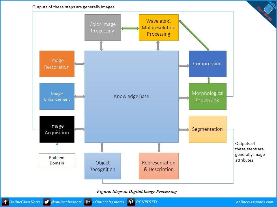
1. Image Acquisition:

This is the first step or process of the fundamental steps of digital image processing. Image acquisition could be as simple as being given an image that is already in digital form. Generally, the image acquisition stage involves pre-processing, such as scaling etc.

2. Image Enhancement:

Image enhancement is among the simplest and most appealing areas of digital image processing. Basically, the idea behind enhancement techniques is to bring out detail that is obscured, or simply to highlight certain features of interest in an image. Such as, changing brightness & contrast etc.

3. Image Restoration:

Image restoration is an area that also deals with improving the appearance of an image. However, unlike enhancement, which is subjective, image restoration is objective, in the sense that restoration techniques tend to be based on mathematical or probabilistic models of image degradation.

4. Color Image Processing:

Color image processing is an area that has been gaining its importance because of the significant increase in the use of digital images over the Internet. This may include color modeling and processing in a digital domain etc.

5. Wavelets and Multi-Resolution Processing:

Wavelets are the foundation for representing images in various degrees of resolution. Images subdivision successively into smaller regions for data compression and for pyramidal representation.

6. Compression:

Compression deals with techniques for reducing the storage required to save an image or the bandwidth to transmit it. Particularly in the uses of internet it is very much necessary to compress data.

Fundamentals of Digital Image Processing

•       Applications of image processing

·       What's an image?

·        A simple image model

·       Fundamental steps in image processing

·       Elements of digital image processing systems

Concept of Sampling

Conversion of analog signal to digital signal:

The output of most of the image sensors is an analog signal, and we can not apply digital processing on it because we can not store it. We can not store it because it requires infinite memory to store a signal that can have infinite values.

So we have to convert an analog signal into a digital signal.

To create an image which is digital, we need to covert continuous data into digital form. There are two steps in which it is done.

• Sampling
• Quantization

We will discuss sampling now, and quantization will be discussed later on but for now on we will discuss just a little about the difference between these two and the need of these two steps.

Basic idea:

The basic idea behind converting an analog signal to its digital signal is

to convert both of its axis (x,y) into a digital format.

Since an image is continuous not just in its co-ordinates (x axis), but also in its amplitude (y axis), so the part that deals with the digitizing of co-ordinates is known as sampling. And the part that deals with digitizing the amplitude is known as quantization.

Sampling.

Sampling has already been introduced in our tutorial of introduction to signals and system. But we are going to discuss here more.

Here what we have discussed of the sampling.

The term sampling refers to take samples

We digitize x axis in sampling

It is done on independent variable

In case of equation y = sin(x), it is done on x variable

It is further divided into two parts , up sampling and down sampling

If you will look at the above figure, you will see that there are some random variations in the signal. These variations are due to noise. In sampling we reduce this noise by taking samples. It is obvious that more samples we take, the quality of the image would be more better, the noise would be more removed and same happens vice versa.

However, if you take sampling on the x axis, the signal is not converted to digital format, unless you take sampling of the y-axis too which is known as quantization. The more samples eventually means you are collecting more data, and in case of image, it means more pixels.

Relation ship with pixels

Since a pixel is a smallest element in an image. The total number of pixels in an image can be calculated as

Pixels = total no of rows * total no of columns.

Lets say we have total of 25 pixels, that means we have a square image of 5 X 5. Then as we have dicussed above in sampling, that more samples eventually result in more pixels. So it means that of our continuous signal, we have taken 25 samples on x axis. That refers to 25 pixels of this image.

This leads to another conclusion that since pixel is also the smallest division of a CCD array. So it means it has a relationship with CCD array too, which can be explained as this.

Relationship with CCD array

The number of sensors on a CCD array is directly equal to the number of pixels. And since we have concluded that the number of pixels is directly equal to the number of samples, that means that number sample is directly equal to the number of sensors on CCD array.

Oversampling.

In the beginning we have define that sampling is further categorize into two types. Which is up sampling and down sampling. Up sampling is also called as over sampling.

The oversampling has a very deep application in image processing which is known as Zooming.

Zooming

We will formally introduce zooming in the upcoming tutorial, but for now on, we will just briefly explain zooming.

Zooming refers to increase the quantity of pixels, so that when you zoom an image, you will see more detail.

The increase in the quantity of pixels is done through oversampling. The one way to zoom is, or to increase samples, is to zoom optically, through the motor movement of the lens and then capture the image. But we have to do it, once the image has been captured.

There is a difference between zooming and sampling

The concept is same, which is, to increase samples. But the key difference is that while sampling is done on the signals, zooming is done on the digital image.

Pixel

We have already defined a pixel in our tutorial of concept of pixel, in which we define a pixel as the smallest element of an image. We also defined that a pixel can store a value proportional to the light intensity at that particular location.

Now since we have defined a pixel, we are going to define what is resolution.

Resolution

The resolution can be defined in many ways. Such as pixel resolution, spatial resolution, temporal resolution, spectral resolution. Out of which we are going to discuss pixel resolution.

You have probably seen that in your own computer settings, you have monitor resolution of 800 x 600, 640 x 480 e.t.c

In pixel resolution, the term resolution refers to the total number of count of pixels in an digital image. For example. If an image has M rows and N columns, then its resolution can be defined as M X N.

If we define resolution as the total number of pixels, then pixel resolution can be defined with set of two numbers. The first number the width of the picture, or the pixels across columns, and the second number is height of the picture, or the pixels across its width.

We can say that the higher is the pixel resolution, the higher is the quality of the image.

We can define pixel resolution of an image as 4500 X 5500.

Megapixels

We can calculate mega pixels of a camera using pixel resolution.

Column pixels (width ) X row pixels ( height ) / 1 Million.

The size of an image can be defined by its pixel resolution.

Size = pixel resolution X bpp ( bits per pixel )

UNIT-II:

Gray Level Transformation

We have discussed some of the basic transformations in our tutorial of Basic transformation. In this tutorial we will look at some of the basic gray level transformations.

Image enhancement

Enhancing an image provides better contrast and a more detailed image as compare to non enhanced image. Image enhancement has very applications. It is used to enhance medical images, images captured in remote sensing, images from satellite e.t.c

The transformation function has been given below

s = T ( r )

where r is the pixels of the input image and s is the pixels of the output image. T is a transformation function that maps each value of r to each value of s. Image enhancement can be done through gray level transformations which are discussed below.

Gray level transformation

There are three basic gray level transformation.

• Linear
• Logarithmic
• Power – law

The overall graph of these transitions has been shown below.

Linear transformation

First we will look at the linear transformation. Linear transformation includes simple identity and negative transformation. Identity transformation has been discussed in our tutorial of image transformation, but a brief description of this transformation has been given here.

Identity transition is shown by a straight line. In this transition, each value of the input image is directly mapped to each other value of output image. That results in the same input image and output image. And hence is called identity transformation. It has been shown below:

Negative transformation

The second linear transformation is negative transformation, which is invert of identity transformation. In negative transformation, each value of the input image is subtracted from the L-1 and mapped onto the output image.

The result is somewhat like this.

Input Image

Output Image

In this case the following transition has been done.

s = (L – 1) – r

since the input image of Einstein is an 8 bpp image, so the number of levels in this image are 256. Putting 256 in the equation, we get this

s = 255 – r

So each value is subtracted by 255 and the result image has been shown above. So what happens is that, the lighter pixels become dark and the darker picture becomes light. And it results in image negative.

It has been shown in the graph below.

Logarithmic transformations

Logarithmic transformation further contains two type of transformation. Log transformation and inverse log transformation.

Log transformation

The log transformations can be defined by this formula

s = c log(r + 1).

Where s and r are the pixel values of the output and the input image and c is a constant. The value 1 is added to each of the pixel value of the input image because if there is a pixel intensity of 0 in the image, then log (0) is equal to infinity. So 1 is added, to make the minimum value at least 1.

During log transformation, the dark pixels in an image are expanded as compare to the higher pixel values. The higher pixel values are kind of compressed in log transformation. This result in following image enhancement.

The value of c in the log transform adjust the kind of enhancement you are looking for.

Input Image

Log Tranform Image

The inverse log transform is opposite to log transform.

Power – Law transformations

There are further two transformation is power law transformations, that include nth power and nth root transformation. These transformations can be given by the expression:

s=cr^γ

This symbol γ is called gamma, due to which this transformation is also known as gamma transformation.

Variation in the value of γ varies the enhancement of the images. Different display devices / monitors have their own gamma correction, that’s why they display their image at different intensity.

This type of transformation is used for enhancing images for different type of display devices. The gamma of different display devices is different. For example Gamma of CRT lies in between of 1.8 to 2.5, that means the image displayed on CRT is dark.

Correcting gamma.

s=cr^γ

s=cr^(1/2.5)

The same image but with different gamma values has been shown here.

For example

Gamma = 10

Gamma = 8

Gamma = 6

Histogram Equalization

We have already seen that contrast can be increased using histogram stretching. In this tutorial we will see that how histogram equalization can be used to enhance contrast.

Before performing histogram equalization, you must know two important concepts used in equalizing histograms. These two concepts are known as PMF and CDF.

They are discussed in our tutorial of PMF and CDF. Please visit them in order to successfully grasp the concept of histogram equalization.

Histogram Equalization

Histogram equalization is used to enhance contrast. It is not necessary that contrast will always be increase in this. There may be some cases were histogram equalization can be worse. In that cases the contrast is decreased.

Lets start histogram equalization by taking this image below as a simple image.

Image

Histogram of this image

The histogram of this image has been shown below.

Now we will perform histogram equalization to it.

PMF

First we have to calculate the PMF (probability mass function) of all the pixels in this image. If you donot know how to calculate PMF, please visit our tutorial of PMF calculation.

CDF

Our next step involves calculation of CDF (cumulative distributive function). Again if you donot know how to calculate CDF , please visit our tutorial of CDF calculation.

Calculate CDF according to gray levels

Lets for instance consider this , that the CDF calculated in the second step looks like this.

Gray Level Value	CDF
0	0.11
1	0.22
2	0.55
3	0.66
4	0.77
5	0.88
6	0.99
7	1

Then in this step you will multiply the CDF value with (Gray levels (minus) 1) .

Considering we have an 3 bpp image. Then number of levels we have are 8. And 1 subtracts 8 is 7. So we multiply CDF by 7. Here what we got after multiplying.

Gray Level Value	CDF	CDF * (Levels-1)
0	0.11	0
1	0.22	1
2	0.55	3
3	0.66	4
4	0.77	5
5	0.88	6
6	0.99	6
7	1	7

Now we have is the last step, in which we have to map the new gray level values into number of pixels.

Lets assume our old gray levels values has these number of pixels.

Gray Level Value	Frequency
0	2
1	4
2	6
3	8
4	10
5	12
6	14
7	16

Now if we map our new values to , then this is what we got.

Gray Level Value	New Gray Level Value	Frequency
0	0	2
1	1	4
2	3	6
3	4	8
4	5	10
5	6	12
6	6	14
7	7	16

Now map these new values you are onto histogram, and you are done.

Lets apply this technique to our original image. After applying we got the following image and its following histogram.

Histogram Equalization Image

Cumulative Distributive function of this image

Histogram Equalization histogram

Comparing both the histograms and images

Conclusion

As you can clearly see from the images that the new image contrast has been enhanced and its histogram has also been equalized. There is also one important thing to be note here that during histogram equalization the overall shape of the histogram changes, where as in histogram stretching the overall shape of histogram remains same.

High Pass vs Low Pass Filters

In the last tutorial, we briefly discuss about filters. In this tutorial we will thoroughly discuss about them. Before discussing about let’s talk about masks first. The concept of mask has been discussed in our tutorial of convolution and masks.

Blurring masks vs derivative masks

We are going to perform a comparison between blurring masks and derivative masks.

Blurring masks

A blurring mask has the following properties.

• All the values in blurring masks are positive
• The sum of all the values is equal to 1
• The edge content is reduced by using a blurring mask
• As the size of the mask grow, more smoothing effect will take place

Derivative masks

A derivative mask has the following properties.

• A derivative mask have positive and as well as negative values
• The sum of all the values in a derivative mask is equal to zero
• The edge content is increased by a derivative mask
• As the size of the mask grows , more edge content is increased

Relationship between blurring mask and derivative mask with high pass filters and low pass filters.

The relationship between blurring mask and derivative mask with a high pass filter and low pass filter can be defined simply as.

• Blurring masks are also called as low pass filter
• Derivative masks are also called as high pass filter

High pass frequency components and Low pass frequency components

The high pass frequency components denotes edges whereas the low pass frequency components denotes smooth regions.

Ideal low pass and Ideal High pass filters

This is the common example of low pass filter.

When one is placed inside and the zero is placed outside , we got a blurred image. Now as we increase the size of 1, blurring would be increased and the edge content would be reduced.

This is a common example of high pass filter.

When 0 is placed inside, we get edges, which gives us a sketched image. An ideal low pass filter in frequency domain is given below.

The ideal low pass filter can be graphically represented as

Now let’s apply this filter to an actual image and let’s see what we got.

Sample image

Image in frequency domain

Applying filter over this image

Resultant Image

With the same way, an ideal high pass filter can be applied on an image. But obviously the results would be different as, the low pass reduces the edged content and the high pass increase it.

Gaussian Low pass and Gaussian High pass filter

Gaussian low pass and Gaussian high pass filter minimize the problem that occur in ideal low pass and high pass filter.

This problem is known as ringing effect. This is due to reason because at some points transition between one color to the other cannot be defined precisely, due to which the ringing effect appears at that point.

Have a look at this graph.

This is the representation of ideal low pass filter. Now at the exact point of Do, you cannot tell that the value would be 0 or 1. Due to which the ringing effect appears at that point.

So in order to reduce the effect that appears is ideal low pass and ideal high pass filter, the following Gaussian low pass filter and Gaussian high pass filter is introduced.

Gaussian Low pass filter

The concept of filtering and low pass remains the same, but only the transition becomes different and become more smooth.

The Gaussian low pass filter can be represented as

Note the smooth curve transition, due to which at each point, the value of Do, can be exactly defined.

Gaussian high pass filter

Gaussian high pass filter has the same concept as ideal high pass filter, but again the transition is more smooth as compared to the ideal one.

Introduction to Frequency domain

We have deal with images in many domains. Now we are processing signals (images) in frequency domain. Since this Fourier series and frequency domain is purely mathematics, so we will try to minimize that math’s part and focus more on its use in DIP.

Frequency domain analysis

Till now, all the domains in which we have analyzed a signal , we analyze it with respect to time. But in frequency domain we don’t analyze signal with respect to time, but with respect of frequency.

Difference between spatial domain and frequency domain

In spatial domain, we deal with images as it is. The value of the pixels of the image change with respect to scene. Whereas in frequency domain, we deal with the rate at which the pixel values are changing in spatial domain.

For simplicity, Let’s put it this way.

Spatial domain

In simple spatial domain, we directly deal with the image matrix. Whereas in frequency domain, we deal an image like this.

Frequency Domain

We first transform the image to its frequency distribution. Then our black box system perform what ever processing it has to performed, and the output of the black box in this case is not an image, but a transformation. After performing inverse transformation, it is converted into an image which is then viewed in spatial domain.

It can be pictorially viewed as

Here we have used the word transformation. What does it actually mean?

Transformation

A signal can be converted from time domain into frequency domain using mathematical operators called transforms. There are many kind of transformation that does this. Some of them are given below.

• Fourier Series
• Fourier transformation
• Laplace transform
• Z transform

Out of all these, we will thoroughly discuss Fourier series and Fourier transformation in our next tutorial.

Frequency components

Any image in spatial domain can be represented in a frequency domain. But what do this frequencies actually mean.

We will divide frequency components into two major components.

High frequency components

High frequency components correspond to edges in an image.

Low frequency components

Low frequency components in an image correspond to smooth regions.

………………………………..

Homomorphic filtering

 is a generalized technique for signal and image processing, involving a nonlinear mapping to a different domain in which linear filter techniques are applied, followed by mapping back to the original domain.

Image restoration tutorial point

Image restoration is performed by reversing the process that blurred the imageand such is performed by imaging a point source and use the point source image, which is called the Point Spread Function (PSF) to restore the image information lost to the blurring process.

Image Restoration is the operation of taking a corrupt/noisy image and estimating the clean, original image. Corruption may come in many forms such as motion blur, noise and camera mis-focus.^[1] Image restoration is performed by reversing the process that blurred the image and such is performed by imaging a point source and use the point source image, which is called the Point Spread Function (PSF) to restore the image information lost to the blurring process.

Image restoration is different from image enhancement in that the latter is designed to emphasize features of the image that make the image more pleasing to the observer, but not necessarily to produce realistic data from a scientific point of view. Image enhancement techniques (like contrast stretching or de-blurring by a nearest neighbor procedure) provided by imaging packages use no a priori model of the process that created the image.

With image enhancement noise can effectively be removed by sacrificing some resolution, but this is not acceptable in many applications. In a fluorescence microscope, resolution in the z-direction is bad as it is. More advanced image processing techniques must be applied to recover the object.

Wiener Filtering

Theory

The inverse filtering is a restoration technique for deconvolution, i.e., when the image is blurred by a known lowpass filter, it is possible to recover the image by inverse filtering or generalized inverse filtering. However, inverse filtering is very sensitive to additive noise. The approach of reducing one degradation at a time allows us to develop a restoration algorithm for each type of degradation and simply combine them. The Wiener filtering executes an optimal tradeoff between inverse filtering and noise smoothing. It removes the additive noise and inverts the blurring simultaneously.

The Wiener filtering is optimal in terms of the mean square error. In other words, it minimizes the overall mean square error in the process of inverse filtering and noise smoothing. The Wiener filtering is a linear estimation of the original image. The approach is based on a stochastic framework. The orthogonality principle implies that the Wiener filter in Fourier domain can be expressed as follows:

Morphological Operations

UNIT-III:

Fourier Series

Fourier series simply states that , periodic signals can be represented into sum of sines and cosines when multiplied with a certain weight.It further states that periodic signals can be broken down into further signals with the following properties.

·         The signals are sines and cosines

·         The signals are harmonics of each other

It can be pictorially viewed as

In the above signal , the last signal is actually the sum of all the above signals. This was the idea of the Fourier.
Discrete Fourier Transform. Discrete Fourier Transform. Thediscrete Fourier transform (DFT) is "the Fourier transform for finite-length sequences" because, unlike the (discrete-space) Fourier transform, the DFT has a discrete argument and can be stored in a finite number of infinite word-length locations.

Transform methods in image processing. An image transform can be applied to an image to convert it from one domain to another. Viewing an image in domains such as frequency or Hough space enables the identification of features that may not be as easily detected in the spatial domain.
DTFT and DFT both are for discrete signal. but, in frequency domain, basicdifference is how many basis vectors you select to represent the signal. in DTFT, frequency axis is continuous which means you take infinite basis vectors.
The DCT, and in particular the DCT-II, is often used in signal andimage processing, especially for lossy compression, because it has a strong "energy compaction" property: in typical applications, most of the signal information tends to be concentrated in a few low-frequency components of the DCT.
The Haar-wavelet transform in digital image processing: its status and achievements. Image processing and analysis based on the continuous or discrete image transforms are classic techniques. The image transforms are widely used in imagefiltering, data description, etc.